4 minutes
Percentage coverage of satellite imagery over region of interest
Earth Engine tricks: Satellite imagery coverage over a region of interest
In my work with Google Earth Engine, over the last few months, I like to believe that I have learnt a few tricks to interact with it. I recently received a query about finding the percentage coverage of satellite imagery over a region of interest. In this post, I would like share a robust approach towards this problem.
~TLDR
I use ee.Image.reduceToVectors() to convert images to ee.FeatureCollection(). Then I simply sum the total area of the collection and find the % coverage.
Explanation
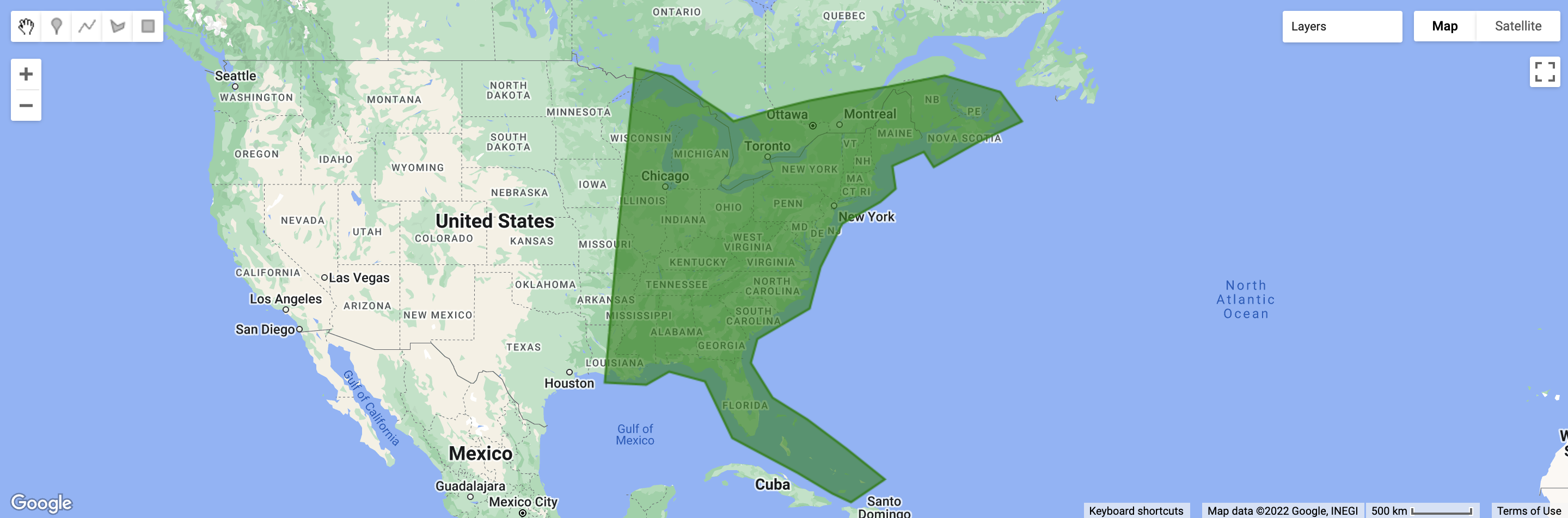
Consider the following large region of interest covering the eastern coast of North America.
var geo = ee.Geometry.Polygon([[-92.52413532482498,29.068796610642462],[-89.18455628452989,28.914934845703456],[-87.33896350523439,29.833880931200852],[-84.43882690085657,29.145338554288642],[-82.24181129937064,25.078787199542987],[-76.96873224229702,22.505730359809384],[-74.15638961145261,20.954634119919458],[-72.61837753681915,20.296610892350177],[-69.93789091531232,22.017775662520798],[-76.17776624731441,26.42435799592542],[-78.99005257253476,27.987520768911722],[-80.74769589300101,30.441776535545372],[-80.22037485372631,32.094264391741454],[-76.00200769123495,34.154844709247236],[-75.12320016955083,36.87260703790422],[-73.36561096544423,39.63248806420696],[-70.28983921701152,40.97286069808757],[-69.05954874360211,41.76428108977483],[-69.32323127521587,43.12600140897638],[-66.77478039524175,43.95416885980774],[-65.9838286583204,43.06190207518716],[-58.86583883168352,45.699391313240426],[-60.62353801334703,47.33193089878859],[-65.10533579067283,48.21761281648529],[-69.58702361515375,47.62863414289759],[-82.17543615981589,45.683704906902776],[-82.83450615124401,46.08134637079505],[-84.59202315164083,46.89813657607063],[-87.06195698922187,48.14757501580384],[-90.06226008975369,48.62591472970412]])
Map.addLayer(geo, {'color': 'green'})
Here is the region of interest.
I will now query Sentinel-2 for some satellite imagery over the region of interest.
var s2_col = ee.ImageCollection('COPERNICUS/S2_SR')
.filterDate('2019-08-30', '2019-09-15')
.filter(ee.Filter.lte('CLOUDY_PIXEL_PERCENTAGE', 20))
.filterBounds(geo)
Typically, over a large area, multiple swaths of the same satellite cover the region of interest in the same day. To produce an easier-to-discern image collection, I like to mosaic the collection over unique dates. This also provides us with much larger images to work with, and thus demonstrate the method well.
var s2_col_list = s2_col.toList(s2_col.size())

var unique_dates_s2 = s2_col_list.map(function(image) {
  return ee.Image(image).date().format('YYYY-MM-dd')
}).distinct()

var mosaick_s2 = unique_dates_s2.map(function(date) {
  date = ee.Date(date)
  return s2_col.filterDate(date, date.advance(1, 'day')).mosaic()
})
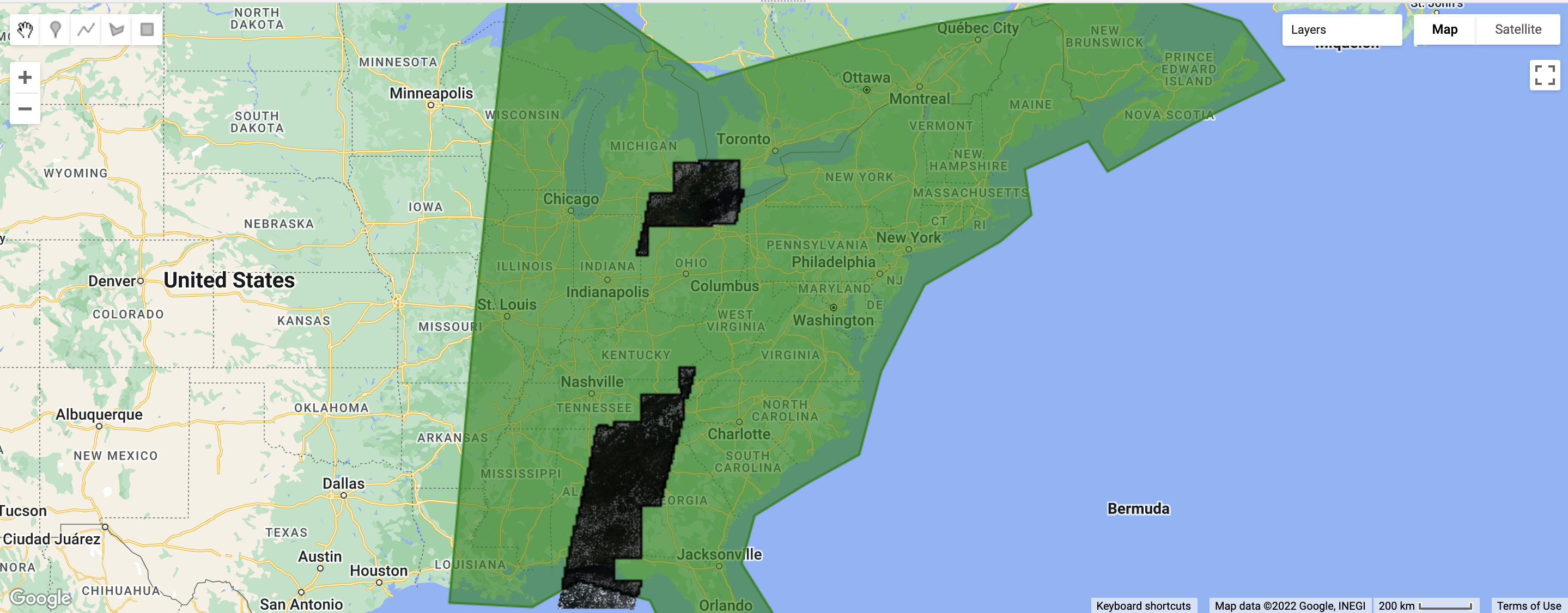
Alright, now that we have prepared our images, we find the features of an image from the image collection. I arbritarily took the 3rd image. You can choose any you like.
var img = ee.Image(mosaick_s1.get(3))
var img_abs = img.abs()
var img_true = img_abs.and(img_abs)
var features = img_true.select('B4').cast({'B4': 'uint32'}).reduceToVectors({'scale': 10000, 'geometry': geo})

Map.addLayer(img, {'bands': ['B4', 'B3', 'B2'], 'min': 0, 'max': 3000})
Map.addLayer(features)
Here are the image and the corresponding regions of interest.
Now we find the total area of features. This revolves around the ee.FeatureCollection().aggregate_sum() method, which finds the sum of a property of the individual features of the collection. So we first create a property area, and assign to it the area of the feature. Then we simply run aggregate_sum() over the feature collection and get the total area.
features = features.map(function(feature) {
  return feature.set('area', feature.area(ee.ErrorMargin(1)));
})

var sum = features.aggregate_sum('area')
Now, its a simple ‘find the percentage’ problem :). I find the ratio of the area of the feature collection to the area of the region of interest and multiply by 100.
var geo_area = geo.area(ee.ErrorMargin(1)) // the area of the region of interest
var ratio = sum.divide(geo_area).multiply(100)

print('Area covered by image', sum)
print('Area of the region of interest', geo_area)
print('% area covered', ratio)
Which gives me the following output:
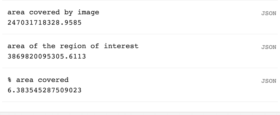
Ofcourse, outputs could be beautified, but as such the areas are in square meters, (a quirk of the ee.geometry.area() function) and can be modified by ee.Number.divide(1000000) to represent square kilometers instead.
The final code here:
var geo = ee.Geometry.Polygon([[-92.52413532482498,29.068796610642462],[-89.18455628452989,28.914934845703456],[-87.33896350523439,29.833880931200852],[-84.43882690085657,29.145338554288642],[-82.24181129937064,25.078787199542987],[-76.96873224229702,22.505730359809384],[-74.15638961145261,20.954634119919458],[-72.61837753681915,20.296610892350177],[-69.93789091531232,22.017775662520798],[-76.17776624731441,26.42435799592542],[-78.99005257253476,27.987520768911722],[-80.74769589300101,30.441776535545372],[-80.22037485372631,32.094264391741454],[-76.00200769123495,34.154844709247236],[-75.12320016955083,36.87260703790422],[-73.36561096544423,39.63248806420696],[-70.28983921701152,40.97286069808757],[-69.05954874360211,41.76428108977483],[-69.32323127521587,43.12600140897638],[-66.77478039524175,43.95416885980774],[-65.9838286583204,43.06190207518716],[-58.86583883168352,45.699391313240426],[-60.62353801334703,47.33193089878859],[-65.10533579067283,48.21761281648529],[-69.58702361515375,47.62863414289759],[-82.17543615981589,45.683704906902776],[-82.83450615124401,46.08134637079505],[-84.59202315164083,46.89813657607063],[-87.06195698922187,48.14757501580384],[-90.06226008975369,48.62591472970412]])
Map.addLayer(geo, {'color': 'green'})

// added geo

var s2_col = ee.ImageCollection('COPERNICUS/S2_SR')
.filterDate('2019-08-30', '2019-09-15')
.filter(ee.Filter.lte('CLOUDY_PIXEL_PERCENTAGE', 20))
.filterBounds(geo)

// created the collection

var s2_col_list = s2_col.toList(s2_col.size())

var unique_dates_s2 = s2_col_list.map(function(image) {
  return ee.Image(image).date().format('YYYY-MM-dd')
}).distinct()

var mosaick_s2 = unique_dates_s2.map(function(date) {
  date = ee.Date(date)
  return s2_col.filterDate(date, date.advance(1, 'day')).mosaic()
})

// mosaiked the collection by date

var img = ee.Image(mosaick_s1.get(3))
var img_abs = img.abs()
var img_true = img_abs.and(img_abs)
var features = img_true.select('B4').cast({'B4': 'uint32'}).reduceToVectors({'scale': 10000, 'geometry': geo})

Map.addLayer(img, {'bands': ['B4', 'B3', 'B2'], 'min': 0, 'max': 3000})
Map.addLayer(features)

// retrived image from mosaiked list and created vectors

features = features.map(function(feature) {
  return feature.set('area', feature.area(ee.ErrorMargin(1)));
})

var sum = features.aggregate_sum('area')

// found sum of areas of features

var geo_area = geo.area(ee.ErrorMargin(1)) // the area of the region of interest
var ratio = sum.divide(geo_area).multiply(100)

print('Area covered by image', sum)
print('Area of the region of interest', geo_area)
print('% area covered', ratio)
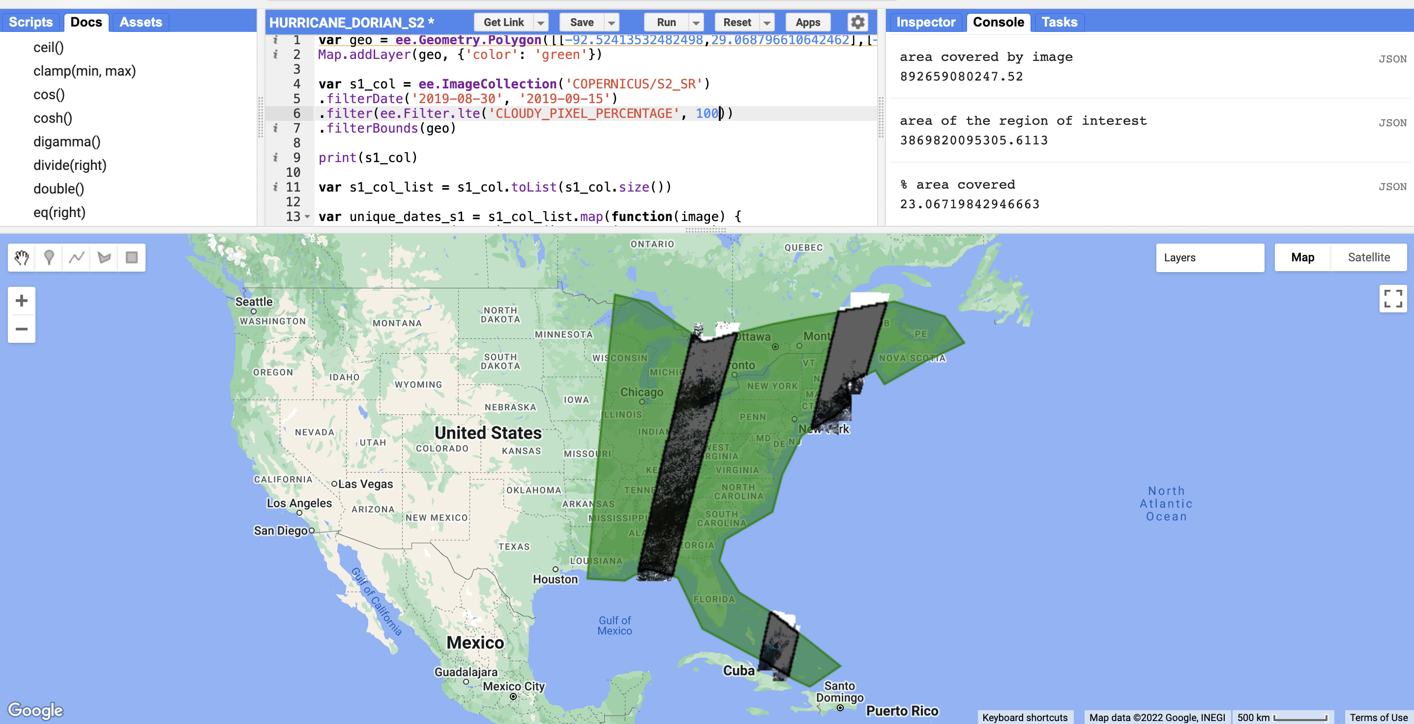
Changing the cloud cover tolerance to 100 gives us more satellite imagery and a larger percentage coverage.
Conclusion
In summary, we learnt how to use reduceToVectors() along with aggregate_sum() to come up with a robust approach towards calculating percentage of area covered by an image.